Using the Optimizer

With the actuator saturations acquired, I was able to put together the following model and optimizer code.

Model

A constant reference of 0, is compared with the gain of the plant to determine an actuation signal representing an acceleration to be applied at the base. This command signal is passed through the actuators subsystem block to apply the actuator dynamics. This potentially saturated signal is passed into the plant state-space model block. The state variables are read from the plant, sent to the workspace, and passed to the controller gains. While running this model, the evolutionary optimizer will be modifying the controller gains and testing the state output.

Let's take a closer look at the actuators subsystem.

The actuators subsystem block takes in a raw acceleration signal and saturates it. This saturated signal is integrated to find the approximate velocity and saturates it as well. If the speed becomes saturated, the acceleration value outputted if forced to 0 via If and If Action blocks. Otherwise, the saturated acceleration value is outputted. The saturated velocity is sent to a Terminator block to prevent a compiler warning and allow the signal to be attached to a scope.

Optimizer

This model is operated by the particle swarm optimizer to find optimal gains for the controller. The evolutionary algorithm is split over three files. The first, simplebalance_env.m, initializes the environment to run the other files.

%
% SimpleBalance - Environment
%
% This file prepares the environment for the simplebalance model files
%

% clear the environment
clear all

% initialize constants
g = 9.81;        % m/s^2, acceleration due to gravity
l = .11125;      % m, length of moment arm
m = 652.039032;  % g, mass of point
M = 28.3495231;  % g, mass of base

% calculate the state-space matrices
A = [0 1; m*g*l/(2*m*l^2) 0];
B = [0; M*l/(2*m*l^2)];
C = [1 0; 0 1];
D = [0;0];

% calculate a conversion factor from rotations to meters.
deg2m = 1/360    * 81.6*pi * 1/1000;
%       rot/deg    mm/rot    m/mm

% calculate the saturation of the motors
velo_top = 900 * deg2m;  % m/s, maximum motor velocity at max battery
accel_top = 200 * deg2m; % m/s^2, maximum motor acceleration at max battery

% set an initial state for the model
x_0 = [.0001;0];

% set an initial gain for the model (so we don't get compiler warnings
% while we're working with it)
K = [0 0];

The inline comments explain most of what's going on. Note that the state equations and constants were determined from my earlier work on this hardware in 2009. The 81.6 used in the degrees to meters calculation is given from the wheel specifications. And as mentioned earlier, the 900 degrees per second velocity and the 200 degrees per second squared acceleration were determine last week. The initial state is set such that a small error is generated away from balanced to demonstrate to task the control to correct for the error.

After the environment has been set, the optimizer can begin to run. The model algorithm is too long to post here, but is accessible via simplebalance_psoa.m. Please open that file if you'd like to follow along. The algorithm is documented, and I'll refrain from reviewing the operation of the optimizer here as I provided materials to it in an earlier post, but here's a few points of interest.

The parameters for the optimizer were pulled from M. E. H. Pedersen's publication Good Parameters for Particle Swarm Optimization. In it, Pedersen summarizes a number of tuning values that can serve as good starting point values for a number of different configurations. Choosing some basic variables have proved to be sufficient.

The globalBest on lines 75 and 118, and the it on line 80 are intentionally left without a semicolon so the script can output a progress report via lines to the command window. Lines 93 and 102 can be uncommented for a similar effect.

I've noticed much better performance in general (not just with this project) without the bounding that the original algorithm outlines with this project and with others. This could be due to a number of reasons, not the least of which is a search bounds being too small. However, I have found that the optimizer with these Pedersen's recommended parameters perform much better without bounds in general as compared to other tuning values. I'll speak more to this in the final paper.

Finally, this implementation of the optimizer uses the following cost function in simplebalance_cost.m.

%
% SimpleBalance - PSOA Cost Function
%
% This file runs the particle swarm optimizer using the simplebalance_cost
% function as a cost function.
%
% This file is intended to be called from simplebalance_psoa.m.

function cost = simplebalance_cost(position)

% assign the workspace variable K with the position of the particle
assignin('base', 'K', position);

% run the simulation against the gain values
sim('simplebalance2');

% if the simulation is a step response, the cost returned can be the
% settling time.
%info = stepinfo(simout.Data(:,1), simout.Time(:,1));
%cost = info.SettlingTime;

% the cost returned is the absolute value of the last simulated point
cost = abs(simout.Data(501,1));

As with the other files this is documented, so I'll stick to the remarks. My original cost function (commented out) was designed to respond to a step response to the reference value. A cost value was mapped from the settling time. The shorter the settling time, the lower the cost. This worked fine before the modifications to the actuator subsystem model were included. Now the model settles from an unstable initial condition and the cost is the final value after 10 seconds of simulation data points are collected. Although we are not theoretically guaranteed that the model is stable under this condition, it has been my findings that it is. And with the configuration shown here, actually over tunes the gain values.

The evolutionary optimization strategy identifies controller gains of about 19800 and 630. After 10 seconds of simulation the cost is smaller than what can be stored in program memory and is sufficiently small to be zero.

Implementing the Optimized Controller

Using these gains, I set out to program the controller into the hardware and created this model. The main loop is trivial...

The plant is much more interesting...

This plant is based off of my experience with the NXC version. The actuation from the control is sent into a gain to convert the meters per second squared acceleration value into units using degrees. The resulting value is summed with the average speed of the motors as read by the encoders to find the new speed. This speed is passed through an additional gain and set to the motors. Meanwhile, the current gyro sensor value is integrated and sent along with its current value to the output. At the moment no consideration is giving for gyro drift.

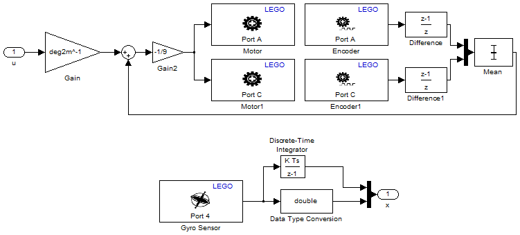
First a few considerations. The gain of 1/9 is required to scale the potential maximum speed of 900 degrees per second to a reasonable motor input signal for the motors between -100 and 100. In reality, this gain would change overtime based on the state of the battery. In a more professional control, there could be another control loop relating motor references, speeds, positions, battery voltages. For this simple model, we ignore those factors. Also, the gain is negated because the motors are mounted backwards to their reference.

Running the model on the hardware leads to jerky attempts to balance. The gyroscopic drift comes back into play as over time the robot believes the balance angle is off from what it should be and is the main source off disturbance. I will continue to investigate this after the project is complete, but I believe the basic tasks set by the proposal to be complete and will focus my attention on the paper.

Modelling Actuator Dynamics

In order to determine gains for the control that will work with the real plant, we will need to take into account some of the actuator dynamics. Unlike in mathematical models, these motors are real, tangible electronics with real world limitations. If we don't take into account the dynamics, the control may not function appropriately, and the robot will not balance.

There are many different dynamics that could be considered to completely model the actuators, in this case, the motors. Internal electronics dynamics, backlash from the transmission, quantization error, and drift all could be included, but for this study, the most restrictive is the motors' maximum velocity and maximum acceleration. If the actuator model includes the saturation effect of these maximums when we use our evolutionary algorithm, the control of the balance will be much more efficient.

Motor Test Model

This past week I was able to put together a simulink model that sampled and recorded the characteristics of one of the motors. Here is that model.

The motor test model, colored for sample rate

This model is colored by sample time. The black is continuous, and the red is 0.01 seconds. Yellow is not applicable. The model is run for 10 seconds.

The current time of the simulation coming from the Clock block is a signal to the If block. The If Action blocks are configured such that the output of the Merge block will be either full forward (100), full reverse (-100) or stopped (0). The If block is configured to snap the motor on port A to full speed in the forward and reverse direction for two seconds each, twice.

At the same time, the signal from the Encoder block for the same motor is read. This block reports the total angle in degrees. Running this signal through a Difference block and a Gain block adjusting for the sample time provides the angular velocity. Doing the same once more provides the angular velocity. These three signals are routed to a Mux block and a To Workspace block to save the information in a workspace variable, "data".

Motor Test Simulation Data

Simulating the model generates the following data points.

The motor test model's simulated data points

In this plot, the rotation (blue), angular velocity (green), and angular acceleration (red) are plotted against time in seconds. Interesting points are labeled with tool tips. The position curve appears smooth as it ramps up and down through the two cycles, but the velocity and acceleration curves amplify the inherent noise. Disregarding filtering, the sampled maximum angular velocity is 900 degrees per second and the sampled maximum angular acceleration 200 degrees per second squared.

NXC Control

Good news! I've been able to get a copy of the latest Matlab with built in support for LEGO Mindstorms components. There have been some obvious short comings with BricxCC that have been hard to overlook. Most importantly, not being able to view the calculated response of the control in real time has become an issue. Also, any information that I can collect through NXT "datalog" files need to go through a spreadsheet utility to be able to analyze. I hope these considerations, as well as the ability to model with the LEGO components themselves, will accelerate my efforts.

But despite my lack of software, I have still been able to make strides in my NXC implementation. There's too much code to paste here, so you'll need to download it if you'd like to follow along. This control is separated into four parallel tasks called getAccelData(), getGyroData(), getButtons(), and setMotorSpeed(). Let's take a look at each one in turn.

setMotorSpeed()

First there's setMotorSpeed(). This code is based off of the control code from a couple weeks ago. In its current state, the code acts as a P controller, and doesn't rely on derivative or integral term. The global values for the ideal angle and the current angle are read, the error is calculated, and run through the control law. The proportional gain is set to 20 by experimentation. The output is then used to set the motor speed as before.

I attempted to use the Ziegler-Nichols method again for tuning, but the gains it provided never lead to the robot coming close to balancing. Instead it would violently oscillate around the equilibrium point. Also, enabling the integral gain with any reasonable value caused the integral term to run away, which I believe to be mostly due to the gyro drift I'll discuss a little later. I decided to disable the Ziegler-Nichols tunings, and the integral term, to try to find a proportional gain that came closed to balancing.

getGyroData()

Before running the getGyroData() task, the initGyro() function is called. This performs the same calibration that I wrote last week.

When getGyroData() is run, the sensors raw value is read. It is filtered into the offset using a weighted sum in a similar manor to the HTWay I analyzed earlier. This regulated value is used as the offset to determine the gyro's actual rotation speed. The speed is integrated into the angle using the approximate time since the last call in the loop. The gyro's offset, speed, and angle are all globals set by this task. Other tasks have read access to them, most importantly, setMotorSpeed().

I had a hard time adjusting the weighting for the filter on the gyro's offset. The value in the HTWay example was set for a configuration different from mine. Since there was little explanation as to how they came to their value, I experimented with values that seemed appropriate. This version of the code has 0.01 which is two orders of magnitude larger that the example's code. I believe this to be necessary due to the different sample rates between the two. Mine is running considerably faster, and may need to be adjusted further.

getAccelData()

This task is actually disabled when compiled as indicated by the first line in the task itself. This was an experiment in resetting the ideal angle for balancing by using the accelerometer, but was unreliable. I believe the idea to be in the right direction, but it's difficult to say.

After initializing the sensor, the tasks main loop begins. The loop reads the accelerometer and calculates the approximate value in Gs experienced in the x (up/down) and the y (forward/backward) directions. It then calculates the derivative of the acceleration, otherwise known as "jerk". Using these values, the ideal angle is reset to the gyro's current sensed angle only if the acceleration in the forward / backward direction is near the value it should be for balancing, and the jerk is near zero indicating the acceleration isn't changing.

I found this to work alright, but it wasn't consistent. Using this method, the upright position can only be detected when the robot is already nearly balanced. If the platform is oscillating around balanced, the ideal angle will never be improved. I haven't tried combining these sensors before, so I figured it might be worth it to take a shot. But since this isn't the focus of this project. I've left this disabled and will move on to something else.

getButtons()

A very simple task, as a debugging alternative, when the left button is held, it constantly resets the ideal angle with the gyro's current angle. This isn't used as part of the control, but was used when testing other components.

Performance

As it operates now, the robot nearly balances, but is effected by the drift of the gyro too much to maintain it's balance. If I run the program and hold the robot in the air nearly balanced, the wheels start stopped but slowly accelerate to full speed in some direction. This gyro drift must be addressed before I can implement a control, with either BricxCC or Matlab.

Looking into the matter more deeply, I came across this forum post on the Mindboards forum, a general Mindstorms discussion board. That particular thread has gone on for nearly a year and has a lot of interesting discussions on the performance and considerations of gyroscopic sensors in general. Most notably for me, it seems that people are able to use the weighted sum without too much trouble. It also obviously works for HiTechnic's example build. There's probably a more appropriate value for that weighting that I haven't found yet.

I'm feeling a little burnt out on this gyro issue for now. Since I have Matlab, I think I'll shift back to exploring the evolutionary algorithms application to this robot.

Shifting to Matlab / Simulink

From my previous work, I already have a model ready to test of a full state feedback controller in the loop with a plant. I could run the evolutionary algorithm over this, but it wont provide much more utility over the existing built-ins with the software (e.g. it's trivial to call Matlab's place or acker to find poles). Instead, I'll try to give the algorithm a more challenging problem by adding some motor dynamics and non-linearities to the the model before proceeding.

Short Week with the Gyro

Once again a big congratulations to FIRST Team 3182, Athena's Warriors for an excellent performance at the Hartford FIRST Robotics Competition! As I'm sure everyone experienced for themselves the past few days, you have a lot to be proud of. Excellent job team! I'm looking forward to next season!

The Gyro

Even though I was occupied at the end of the week with the competition, I was still able to get some work done investigating the gyro thanks to HiTechnic and their very prompt delivery! It's handy to be close to the distribution center! :)

The HiTechnic gyroscopic sensor is a piezoelectric device that is capable of measuring the angular velocity of the sensor in a single plane. By mounting the sensor on the robot in an appropriate orientation, we will be able to replace the accelerometer as a means of detecting the tilt of the robot.

I've modified the original design to mount both sensors for now, with the gyro on the right side of the image (left side of the robot). I've also added some larger wheels for improved velocity at the base. Additional mass these components add is negligible from my earlier measurements. Here's the Mark II platform (Mark I is from 2009).

Mark II platform

Gyro Initialization

Before any reading can be done for the controller, we must first initialize the gyroscopic sensor with an offset value. The following code finds a offset value automatically based on readings from the sensor in a stable location. This code is based on the HTWay's gyro initialization.

// setup some temporary variables
int gyroMin_degPs,
    gyroMax_degPs,
    gyroRaw_degPs,
    gyroSum_degPs;

int it = 0;

float g_gyroOffset_degPs;

SetSensorHTGyro(S4);
Wait(100);

// find the initial gyro offset
do {
  gyroSum_degPs = 0;
  gyroMin_degPs = 1000;
  gyroMax_degPs = -1000;
  for (it = 0; it < 100; it++) {
    gyroRaw_degPs = SensorHTGyro(S4);
    if (gyroRaw_degPs > gyroMax_degPs) {gyroMax_degPs = gyroRaw_degPs;}
    if (gyroRaw_degPs < gyroMin_degPs) {gyroMin_degPs = gyroRaw_degPs;}
    gyroSum_degPs += gyroRaw_degPs;
    Wait(5);
  }
} while ((gyroMax_degPs - gyroMin_degPs) > 1);   // Reject and sample again if range too large

// average the sum of the samples
g_gyroOffset_degPs = gyroSum_degPs / 100.0;

After setting some initial variables, the SetSentorHTGyro() call sets the sensor to be on port 4 of the NXT. The Wait() immediately following it makes sure that the gyro is settled and will not send out garbage data immediately after initializing it. The embedded loops that follow read a raw value from the sensor, update some minimum and maximum values, and sum the raw readings together. This is repeated 100 times. If the minimum and maximum values are too far apart, that process is repeated and a new set of 100 data points are sampled. This guarantees the sensor wasn't moved during the initialization process. If the minimum and maximum values are close enough, the sum is averaged to find the sampled gyro offset.

Gyro Reading

To get an idea of what the drift on the gyro looks like, I put together the following code. This code will prepare a file with 513 records of tick times (milliseconds) and raw readings. While leaving the sensor untouched, any change in the sensor's value is caused by the natural drift.

This code is based on the HTWay's gyro reading code. Note that the offset I determined with the code above isn't used here since I'm most interested in the natural drift of the sensor, not necessarily its drift from a sample.

// setup some temporary variables
int firstTick, lastTick;
int t1, t2, t3, t4;
int i, bytesWritten, tmp;
byte fileHandle;
string buffer;

DeleteFile("gyro_idle.csv");
CreateFile("gyro_idle.csv", 4096*2, fileHandle);

firstTick = CurrentTick();
lastTick = firstTick;
for (i = 0; i <= 512; i++) {
  // read the sensor
  tmp = CurrentTick() - firstTick;
  buffer = StrCat(NumToStr(tmp), ",");
  t1 = CurrentTick();
  tmp = SensorHTGyro(S4);
  buffer = StrCat(buffer, NumToStr(tmp));
  t2 = CurrentTick();
  WriteLnString(fileHandle, buffer, bytesWritten);
  t3 = CurrentTick();
  
  // output timing debug info
  ClearScreen();
  NumOut(10, LCD_LINE1, t1 - lastTick);
  NumOut(10, LCD_LINE2, t2 - t1);
  NumOut(10, LCD_LINE3, t3 - t2);
  t4 = CurrentTick();
  NumOut(10, LCD_LINE4, t4 - t3);
   
  lastTick = CurrentTick();
  Wait((20));
}

CloseFile(fileHandle);

This code begins with initializing temporary variables. Next, a file is deleted and created in preparation for the records to be written to it. After calculating an initial tick value, the main loop is run. For each iteration, a string of the current tick and the current gyro value are concatenated separated by a comma. The resulting string is written to the file. The additional lines dealing with timing are printed to the NXT's LCD screen and used to debug the loop timing. Finally, the loop waits 20 ticks before running again. At its completion, the file is closed for good house keeping.

The Results

The resulting data file can be acquired by using a utility from the BricxCC's NXT Explorer. Without even plotting this data, it's pretty obvious that there are more readings at a -1 value at the start of the test then at the end, but for good measure, here's a plot of the same information.

Raw gyro values at idle

Without a doubt, this drift will need to be accounted for.

Naive Control Test

Now familiar with BricxCC and the HTWay, it's time check the new platform's operation. I'm trying to get as close to a balancing code as possible with an accelerometer, but not worrying about it too much until I acquire the latest Matlab. In the meantime, this should bring to light a lot of other considerations that will need to be evaluated and handled in the final control. To get this naive control to work adequately, I'll try using Ziegler-Nichols tuning on a basic control that maps angle to motor speeds. First, a word on the tuning method.

Ziegler-Nichols Tuning Method

J.G. Ziegler and N.B. Nichols in 1942 published "Optimum Settings for Automatic Controllers" as part of "Transactions of the ASME". In it, Ziegler and Nichols developed time domain and frequency domain methods of determining appropriate tuning values. These values are based off of step response and frequency response characterizations of the system's dynamics. Consisting of relatively simple rules, its easy to apply the method to many different problems. For a complete discussion of Ziegler-Nichols tuning, I suggest looking into the wikipedia article, and the original ASME article republished with permission at http://www.driedger.ca/.

For my process, I decided to follow the frequency response method. I attempted to identify the critical oscillation gain, the gain at which the robot oscillated around the upright balanced position, and the period at which it oscillated. To determine this value, I ran a simplified version of the code below with only the proportional factor controlling the output. I varied the values of the proportional gain until the platform began to oscillate nearly around the point of balancing. I found this value to be 1.25. The period at which it oscillated was estimated to be 200 milliseconds.

Naive Control

After some trial and error I was able to put together the code at the end of this post, a simple implementation of a PID controller in NXC. Let's go through stanza by stanza and I'll explain what's going on, the intent behind the code, and considerations for future implementations.

Lines 1 through 5 defines the bound function. This function returns the value of x bounded by an upper and lower value. Since the motors should only be set with values between -100 and 100, we'll use this to limit its actuation.

Line 7 begins the main task. This is the first task that is run on the NXT. Tasks are similar to threads or parallel processes. We could have multiple tasks for sensing and actuation for potentially better performance. For more complex code, I'll revisit this idea.

Lines 8 through 23 declare the variables needed:

• Integers
• angle - The angle is represented by acceleration expressed in the forward and backward horizontal plane of the robot in gs divided by 200.
• deltaTime - The approximate time between each iteration of the main loop in milliseconds. This is set to be 50. A known delta value is used to control the loop speed so further analysis can take place down the road.
• error - The difference between the idealAngle and the sensed angle in gs divided by 200.
• garbage - Not used for anything constructive. This is necessary when acquiring data from the accelerometer.
• idealAngle - The sensed balanced acceleration value in gs divided by 200. Due to the weight distribution of the hardware, the robot needs to lean a little forward to be balanced. Thus, this is set to 9.
• lastError - The last error value from the last loop iteration in gs divided 200.
• overheadTime - The time in milliseconds the sensor acquisition, calculations, and motor settings need to complete. Using the commented lines, I was able to determine this to be about 16 milliseconds.
• Floats
• derivative and integral - The derivative and integral values from the PID calculations.
• Kc and Pc - The critical oscillation gain and period. Specifically, Kc is the minimum proportional gain necessary to oscillate the system as described in the last second. These are set to 1.25 and 200 respectively.
• Kp, Ki, and Kd - The proportional, integral, and derivative gain values. Note that the derivative gain is set to zero. Derivative terms can add a lot of noise to a system, so this is left out for now.
• output - The output from the PID control.

Lines 25 through 27 initialize the proportional and integral gains using the Ziegler-Nichols tuning method. The critical oscillation gain is multiplied by 0.45 to determine the proportional gain. The proportional gain is multiplied by 1.2 and divided by the period to get the integral gain.

Lines 29 and 30 initialize the accelerometer for reading. This could take some time, so a brief wait is called after the initialization.

Lines 33 through 36 find an initial last error value by reading the accelerometer and finding its difference from the ideal value.

Lines 38 and on are the main loop of the program. All lines that have NumOut(...) are debugging output that gets printed to the NXT's LCD screen.

Line 40 forces the loop to wait an adjusted value to match an actual delay nearly the set delta time.

Lines 49 through 60 find the sensor value and calculate the PID controller's output.

Line 63 sets the motor speed. Note that the output is multiplied by -1.0 because the motors are mounted backwards.

Running the Code

Running the code on the platform has made it apparent the accelerometer alone is not sufficient for balancing. The accelerometer is sensing the acceleration the robot is under. Our axis of interest is the forward-back horizontal direction. In the presence of gravity and no other forces, the acceleration could be directly mapped to an angle accurately. But because the robot is actually under many forces, most importantly the motor driven wheels keeping it balanced, the acceleration in our axis of interest will be the result of all these forces. Another sensor is necessary.

A piezoelectric gyroscope is a sound alternative. Mounted in the appropriate axis, it can be used to detect the speed at which the angle of the robot is changing. This could be used to accurately determine the robot's angle. With more effort, this could be used in conjunction with the accelerometer for even more accurate sensing. I've placed an order for the HiTechnic gyro sensor I discussed in my last post. It should be arriving next week. I'll adjust the controller and try again with the gyroscope.

Next week will be a short week for work on the project. I'll be mentoring the FIRST Robotics Competition Hartford Regional, but I'll try to get as much done as possible.

Source Code

1   int bound(int lower, int x, int upper) {
2     if (x < lower) {return lower;}
3     if (x > upper) {return upper;}
4     return x;
5   }
6

7   task main() {
8     unsigned long tick;
9     int angle,
10        deltaTime = 50, // must be >16
11        error,
12        garbage,
13        idealAngle = 9,
14        lastError,
15        overheadTime = 16;
16    float derivative, 

17          integral = 0,
18          Kc = 1.25,
19          Kp = 0,
20          Ki = 0,
21          Kd = 0,
22          output,
23          Pc = 200.0;
24     
25    Kp = 0.45 * Kc;
26    NumOut(10, LCD_LINE1, Kp);
27    Ki = 1.2 * Kp * deltaTime / Pc;
28     
29    SetSensorLowspeed(S4);
30    Wait(50);
31
32    // read sensor (15 ticks)
33    ReadSensorHTAccel(S4, angle, garbage, garbage);
34  

35    // set an initial last error
36    lastError = idealAngle + angle;
37
38    while (true) {
39      // wait
40      Wait(deltaTime - overheadTime);
41     
42      NumOut(10, LCD_LINE1, Kp, DRAW_OPT_CLEAR_WHOLE_SCREEN);
43      NumOut(10, LCD_LINE2, Ki);
44      NumOut(10, LCD_LINE3, Kd);
45     
46      //tick = CurrentTick();
47 
48      // read sensor (15 ticks)
49      ReadSensorHTAccel(S4, angle, garbage, garbage);

50 
51      // pid calculations (0 ticks)
52      error = idealAngle - angle;
53      NumOut(10, LCD_LINE4, error); 

54      integral = integral + (error * deltaTime);
55      NumOut(10, LCD_LINE5, integral);
56      derivative = (error - lastError) / deltaTime;
57      NumOut(10, LCD_LINE6, derivative); 

58      output = (Kp * error) + (Ki * integral) + (Kd * derivative);
59      NumOut(10, LCD_LINE7, output);
60      lastError = error;
61   
62      // set motor speed (0-1 tick)
63      OnFwdSync(OUT_AC, bound(-100, output * -1.0, 100), 0);
64   
65      //NumOut(10, LCD_LINE1, CurrentTick()-tick);
66    }
67  }

BricxCC and HTWay Analysis

Now that I've identified BricxCC is a workable environment, it's worth looking into a bit deeper. Bricx Command Center, or BricxCC for short, is an integrated development environment for programming LEGO microcontrollers, such as the NXT. It provides a lot of great tools for operating the NXT. I've found a lot of utility with the direct control tool, the file explorer, and the register watcher while experimenting deploying code to the NXT. I also came across a very interesting similar project online that's worth comparing parallels with.

HiTechnic's "HTWay"

HiTechnic, a 3rd party sensor manufacturer for the Mindstorms platform, has also created a self balancing robot. Here's a video overview of their design in action.



Their robot is similar in design to what I'm working with. At it's heart, it build from LEGO Mindstorms components including the NXT. Their version is more complex including remote control via a infrared remote, and they have added considerations for when the robot has fallen over, and allows you to adjust the wheel sizes when starting the program for the first time. They are also using a gyroscope to detect their robot's tilt angle and velocity. For more information on the HTWay, take a look at their blog page, which also has links to build instructions and code in different languages.

HTWay Control Law

From the NXC code, here is the control law that keeps this balanced.

power = (KGYROSPEED * gyroSpeed + // Deg/Sec from Gyro sensor
    KGYROANGLE * gyroAngle) / ratioWheel + // Deg from integral of gyro
    KPOS * motorPos + // From MotorRotaionCount of both motors
    KDRIVE * motorControlDrive + // To improve start/stop performance
    KSPEED * motorSpeed; // Motor speed in Deg/Sec

The control law takes the gyro's velocity and angle as well as the motor rotation and velocity. The variable motorControlDrive is used as part of the remote control system of the robot. For this analysis it can be considered equal to zero since my project doesn't include any remote control. The gains, set as macros, are given and not calculated. There's no background information as to how those were chosen that I came across.

The state space model that my hardware is based off of, originally discussed in 2009, is very similar to this. My state is defined as the derivative to angle and the angle itself, as they have in their control respectively. This is promising that this is a sound state to be using. And in fact, if I were concerned with where the robot was, or how fast it was traveling, I could also add the position and velocity of the base. Since I'm not doing any remote control, this can be neglected, and left perhaps as an opportunity for expansion later on.

Sensor Considerations

Another interesting piece of information that has come out of this evaluation has to do with the gyroscope. When the gyroscope is run over time, it tends to drift. One way of combating this is using a filter before determining the angle. The NXC code for this on the HTWay is this.

gyroRaw = SensorHTGyro(GYRO);
gOffset = EMAOFFSET * gyroRaw + (1-EMAOFFSET) * gOffset;
gyroSpeed = gyroRaw - gOffset;

gAngleGlobal += gyroSpeed*tInterval;
gyroAngle = gAngleGlobal;

In this code, the raw value from the gyroscope is read, then passed through a filter in the form of a weighted sum to determine the "true" offset. The offset is used in calculating the speed of rotation. The macro EMAOFFSET is given as 0.0005 and not calculated. Conceptually, the majority of the "influence" over the "true" offset value is driven by the previous value of the offset. This further enlightened me to the fact that sensors are faulty and need to be accommodated.

Unfortunately, I only have an accelerometer on hand. I will attempt to work with it before ordering a gyroscope. If it comes to using a gyroscope for tilt angle calculations, I will attempt to leverage the accelerometer I have to aid in the gyro's drift accommodations.

Short Week on the Environment

Thursday, Friday, and Saturday of this week I was in Worcester for the FIRST Robotics Competition, WPI Regional. A big congratulations to FIRST Team 3182, Athena's Warriors, for placing 5th and making it to the first round of the finals. Excellent job team! Let's keep it up for Hartford at the end of the month! :)

Environment Work

Even though my focus shifted to FIRST at the end of the week, I was still able to begin preparations of my environment for programming the NXT. It was painfully obvious during my first LEGO project that the environment provided by LEGO was not robust enough to handle my needs. Despite being based off of LabView, the simplified interface did not provide enough utility to perform advanced functions.

Matlab and Simulink are going to be a big part of this project, so without a doubt this is the desired interface. Fortunately, Matlab 2012a includes libraries for the NXT and it's most popular accessories. Unfortunately, my computer has 2010a. It is possible to use RWTH, another NXT toolbox, with this older MATLAB version, but all my efforts haven't been able to configure this correctly. For now, when I try to run Comm_OpenNXT from the command window to begin communicating with the NXT, the function returns the following error. The NXT is attached appropriately and has been reset. Tracking this down online hasn't turned up anything useful either.

No NXT found on USB bus! Make sure the NXT is turned on and access rights in /dev/ are
properly set. Rebooting your NXT might help!

Rather than lose more time on RWTH, I decided to begin experimenting with BricxCC while I get a copy of the latest Matlab. BricxCC is an integrated development environment for working with NXTs as well as many other hobbyist controllers. In this environment, an NXT is programmed in a language called "Not Exactly C" (NXC), which borrows a lot from C, but has a much more narrow, restricted focus on NXT programming and includes a very substantial API. For example, NXC introduces a new keyword task which when managed correctly allows the programmer to easily create parallel threads.

So far I have been able to install the software and compile a basic program. Next week I will look into writing meaningful code and deploying it to the NXT.

Project Registration

I stopped into the Registrars Office this week to see Dottie. She helped me finish my project registration and gave me some other graduation materials as well. I am now registered for the project and will prepare my graduation materials soon.